Feeds:
Posts
Comments

Archive for the ‘Programming in Linux’ Category

Jupyter Notebook is part of Project Jupyter which is announced by Fernando Pérez in 2014. It’s a spin-off project from IPython and become the kernel for Jupyter.
Jupyter is a language agnostic and support other programming language like Python, Julia, R, Haskel and Ruby. It’s 100% open-source.
The file format for Jupyter is ‘.ipynb’.
The Jupyter kernel is responsible for handling various type of request (code execution, code completion, inspection) and providing a reply. Since it can connect to many kernels,
it can provide programming in different languages.

In this tutorial, I use:
-Xubuntu 18.04
-Docker 20.10.14

STEP1.FIND THE IMAGES
First, we have to get the docker image. Make sure you are connected to the Internet.

darklinux@darklinuxpc:~$ docker search jupyter
NAME                                   DESCRIPTION                                     STARS     OFFICIAL   AUTOMATED
jupyter/datascience-notebook           Jupyter Notebook Data Science Stack from htt…   917                  
jupyter/all-spark-notebook             Jupyter Notebook Python, Scala, R, Spark, Me…   375                  
jupyter/scipy-notebook                 Jupyter Notebook Scientific Python Stack fro…   340                  
jupyterhub/jupyterhub                  JupyterHub: multi-user Jupyter notebook serv…   310                  [OK]
jupyter/tensorflow-notebook            Jupyter Notebook Scientific Python Stack w/ …   301                  
jupyter/pyspark-notebook               Jupyter Notebook Python, Spark, Mesos Stack …   224                  
jupyter/base-notebook                  Small base image for Jupyter Notebook stacks…   169                  
jupyter/minimal-notebook               Minimal Jupyter Notebook Stack from https://…   154                  
jupyter/r-notebook                     Jupyter Notebook R Stack from https://github…   44                   
jupyterhub/singleuser                  single-user docker images for use with Jupyt…   43                   [OK]
jupyter/nbviewer                       Jupyter Notebook Viewer                         27                   [OK]
bitnami/jupyter-base-notebook                                                          24                   
jupyterhub/k8s-hub                                                                     18                   
bitnami/jupyterhub                                                                     11                   
jupyterhub/k8s-singleuser-sample                                                       9                    
jupyterhub/configurable-http-proxy     node-http-proxy + REST API                      6                    [OK]
jupyterhub/k8s-network-tools                                                           2                    
graphcore/pytorch-jupyter              The Poplar® SDK plus PyTorch for IPUs includ…   1                    
ibmcom/jupyter-base-notebook-ppc64le   Small base image for Jupyter Notebook stacks…   1                    
pachyderm/jupyterhub-pachyderm-user                                                    0                    
ibmcom/jupyter-nb-nb2kg                                                                0                    
pachyderm/jupyterhub-pachyderm-hub                                                     0                    
graphcore/tensorflow-jupyter           The Poplar® SDK plus TensorFlow 1 & 2 for IP…   0                    
ibmcom/jupyter-ppc64le                                                                 0                    
ibmcom/jupyter                                                                         0                    
darklinux@darklinuxpc:~$
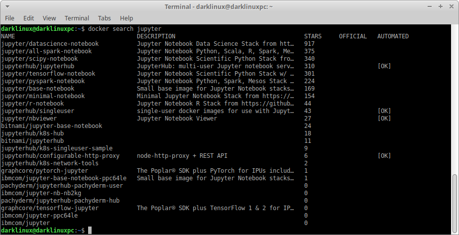
(more…)

Read Full Post »

Getting Market Stock Data from Yahoo Finance is not difficult with Python Module – Pandas.
To follow this tutorial at least you know how to run python code.
In this tutorial, I use:
-Python 3.6.9 (default, Dec 8 2021, 21:08:43)
-Matplotlib-3.3.4
-Pandas 1.1.5
-Xubuntu 18.04
and Vim for text editor

Before you start, make sure you are connected to the Internet.

If you don’t have Python, Matplotlib and Pandas, you can install it from Linux Terminal with commands below:

$ sudo apt-get install python3
$ pip3 install matplotlib
$ pip3 install pandas

The source codes:

(more…)

Read Full Post »

What is Reverse Engineering?

It’s a decompilation of an application so we learn how it work, find the bug or modify it.
Software developer use it for exploit their software weaknesses and strengthen its defenses.
Hackers use it to expose security holes and take advantages of it.

Breaking something down and putting it back together is a process that helps people understand how things were made. Reverse engineering is a way for us to understand how things were designed, how it works, and what its purpose is. In effect, the information is used to redesign and improve for better performance and cost. It can even help fix defects.

In order to understand how it work, at least you have to know a basic knowledge in Assembly Language and Debugging Tools. Regardless what programming language that was used to make the application, at the end it has to be compiled into a machine code before it can run on the computer. Because computer only know machine code.

And to understand the machine code, once again you need to know Assembly Language.

If you want to learn more about reverse engineering, I suggest you to start with small program in c, debug it and observe how it work. Why c? Because c is close to Assembly. If you are not familiar with Assembly and Gdb, I wrote some articles about it also, so you can read it as reference.

One more thing, since in this tutorial I use Vim as hexadecimal editor, you have to know basic knowledge about Vim also. Vim is a text editor but it has a capability to convert a program to hexadecimal and edit the content.

Let’s start.

In this tutorial, I use:
-Xubuntu 18.04
-GNU gdb 8.1.1
-gcc version 7.5.0
-vim version 8.0.1453

Below, is the simple code that we will use for the practice. It’s written in c language. We will use gcc as the compiler.
The program is very simple, the process are:
-Display message ‘Enter your password’
-Check the input password.
-If it is equal, display ‘Access Granted’.

-If it is not equal, display ‘Wrong passwod’.
-then exit

#include<stdio.h>
#include<string.h>

void granted();

int main()
{
  char password[16];
  printf("Enter your password: ");
  gets(password);
  
  if (strcmp(password,"passwordkey"))
  {
  	printf("\nWrong password!\n");
  }
  else
  {
  	granted();
  }
}

void granted()
{
	printf("\nAccess granted!\n");
	return;
}

What we will do to the program is we change the sequence.
Any input for password that is not equal, display ‘Access Granted’.

Read Full Post »

I try to make comparison about Memory Layout between x86-32 bit and x86-64 bit in Linux.

I run 3 different programs, code written in Assembly, C language and python to see how they are loaded into the memory. Then each program I make another 2 copy. So, each language will represent 3 programs.

I use tmux in Linux Terminal, so we can see all programs run together.

Before we start, you have to know the concept behind memory layout in Linux so you will understand what I’m going to explain in this article.

Memory Layout in Linux
For Architecture 32 bit, at the time a program is loaded into memory, all sections of the programs are loaded into each part of the memory. All codes and data which are declared all brought together, even if the source code is separated. The instruction in .text section is loaded into address 0x0804800. Followed by .data section and .bss section. The last address of linux is 0xbFFFFFF.

See the picture below:
memlayout00

In this tutorial, I use AMD processor (Intel compatible). Since the byte order use Little Endian which is start with LSB (lowest significant byte), we have to read the memory from bottom to up.

Virtual Memory Organized
If all programs are loaded in the same location in the memory, why it never over lap each other?
It’s because the program only access the Virtual Memory.
Physical Memory is RAM chip of your computer.
Virtual Memory is the way program think about the memory.
Before a program is loaded in a memory, Linux will search for the empty physical memory that big enough to hold the program. Then it will tell processor to pretend that this memory address is real address of 0x08048000 for the program to stay. After that each program will have it’s own sandbox to play.

Every program will believe that they are stand alone and enjoy all they memory that they have.
So, the address that program believe to use is named Virtual Address meanwhile the real address in the memory chip is named Physical Address.
Process that pointed virtual address to physical address is named Mapping.

Multi tasking in Linux
The Core of Linux is a Block Code that is name Kernel. Memory System is marked as Kernel Space and User Space. Communication in between is handled by System Call. Access to Hardware is limited in software that is run in Kernel Space and only can be done via Kernel Mode Device Drivers.

VDSO (Virtual Dynamically Linked Share Object).
VDSO is memory area allocated in user space for kernel functionalities purpose. It’s kernel mechanism that is used for program to call Kernel Space routines. VDSO use standard mechanism for linking and loading ELF format (Executable and Linkable Format).

(more…)

Read Full Post »

Pandas in Python Library that is used for Data Manipulation and Analysis. It came from terms “Panel Data”. It’s open source under three-clause BSD License. Original developer was Wes McKinney in 2008 while he worked at AQR Capital Management to process Quantitative Analysis on financial data. It was written in Python, Cython and C.

Pandas in mainly used for Machine Learning.

There a lot of features available that you can used for:
-reading and writing various data format, csv, MS excel, json, html, SAS, SPSS, SQL, Google Big Query, Stata, Msgpack etc.
-Group, Join, Merge, Filter, Pivot, Reshaping data set.
-Time series function and so many more.

Installation
In this tutorial I use Python 3.6.9 (default, Nov 7 2019, 10:44:02), so the installation command will be: pip3 install pandas.
From Linux terminal type:

$ pip3 install pandas
Collecting pandas
  Downloading https://files.pythonhosted.org/packages/bb/71/8f53bdbcbc67c912b888b40def255767e475402e9df64050019149b1a943/pandas-1.0.3-cp36-cp36m-manylinux1_x86_64.whl (10.0MB)
    100% |████████████████████████████████| 10.0MB 48kB/s 
Collecting python-dateutil>=2.6.1 (from pandas)
  Using cached https://files.pythonhosted.org/packages/d4/70/d60450c3dd48ef87586924207ae8907090de0b306af2bce5d134d78615cb/python_dateutil-2.8.1-py2.py3-none-any.whl
Collecting numpy>=1.13.3 (from pandas)
  Downloading https://files.pythonhosted.org/packages/07/08/a549ba8b061005bb629b76adc000f3caaaf881028b963c2e18f811c6edc1/numpy-1.18.2-cp36-cp36m-manylinux1_x86_64.whl (20.2MB)
    100% |████████████████████████████████| 20.2MB 45kB/s 
Collecting pytz>=2017.2 (from pandas)
  Using cached https://files.pythonhosted.org/packages/e7/f9/f0b53f88060247251bf481fa6ea62cd0d25bf1b11a87888e53ce5b7c8ad2/pytz-2019.3-py2.py3-none-any.whl
Collecting six>=1.5 (from python-dateutil>=2.6.1->pandas)
  Using cached https://files.pythonhosted.org/packages/65/eb/1f97cb97bfc2390a276969c6fae16075da282f5058082d4cb10c6c5c1dba/six-1.14.0-py2.py3-none-any.whl
Installing collected packages: six, python-dateutil, numpy, pytz, pandas
Successfully installed numpy-1.18.2 pandas-1.0.3 python-dateutil-2.8.1 pytz-2019.3 six-1.14.0
$

pandas01
(more…)

Read Full Post »

It’s fun that Math formula can visualize ‘LOVE’ word.
Type the code below in your python IDE and run it.

import matplotlib.pyplot as plt
import numpy as np
L=np.arange(0,6,0.1)
O=np.arange(-3,3,0.1)
V=np.arange(-2,3,1)
E=np.arange(-3,3,0.1)
fig,(ax1,ax2,ax3,ax4)=plt.subplots(ncols=4)
ax1.set_title(r'$ y=\frac{1}{x}$') #display Math formula
ax1.plot(L,1/L)                    #print L
ax2.set_title(r'$ x^2+y^2=9$')     #display Math formula
ax2.plot(O,(9-O**2)**0.5)          #print O
ax2.plot((9-O**2)**0.5,O)
ax2.plot(O,-(9-O**2)**0.5)
ax3.set_title(r'$ y=|-2x| $')      #display Math formula
ax3.plot(V,(abs(-2*V)))            #print V
ax4.set_title(r'$ -3|sin y| $')    #display Math formula
ax4.plot(-3*abs(np.sin(E)),E)      #print E
plt.show()

love-code
love

Read Full Post »

Pie is very useful to visualize relative proportions of a data set and easily to be understood. The size of the circle will calculated based on the total quantity it represents.
pie01
For example:
There are 3 color in a cirlce, Grey 25, Blue 25 and Green 50.
So total circle size is: 25+25+50=100
The size for the color will be:

Grey  → 25/100 = 0.25 x 100% = 25%
Blue  → 25/100 = 0.25 x 100% = 25%
Green → 50/100 = 0.25 x 100% = 50%

Let’s say the size total is not 100, Grey 30, Blue20 and Green 40.
The total size is: 30+20+40=90.
What the percentage will be?

Grey → 30/90 = 0.3333 x 100% = 33.33%
Blue → 20/90 = 0.2222 x 100% = 22.22%
Green → 40/90 = 0.4444 x 100% = 44,44%

pie02
(more…)

Read Full Post »

Histogram is also a bar type graph chart. The main different between Bar Chart and Histogram Chart are:
Bar Chart for compare numeric data among Categories.
Histogram Chart for compare numeric data in a Category which is distributed into ‘bin’ or ‘bucket’. The term of ‘bin’ in here is a group data.

For example:
you have 24 population in a town with age below:

5,6,7,5,6,4,10,15,14,13,30,35,23,36,45,49,40,51,55,53,60,65,66,70

and you want to visualize it into a graph.

Let’s try.
Open your python IDE and type the code below.

import matplotlib.pyplot as plt
age=[5,6,7,5,6,4,10,15,14,13,30,35,23,36,45,49,40,51,55,53,60,65,66,70]
plt.hist(age)
plt.show()

hist01
hist02

(more…)

Read Full Post »

Older Posts »